Uncertainty

This website is no longer maintained. Please be aware that the content may be out of date or inaccurate. If you have any questions get in touch.

Written by Andy Connelly. Published 16th May 2017. Updated on 16th July 2017.

Introduction

The most effective way to measure the uncertainty associated with a set of results is to repeat measurements. Each repeated measurement of a sample will give you a slightly different result and based on the variation in these results you can then calculate the uncertainty of the average (mean) of those results. This uncertainty gives you, and anyone looking at your data, an indication of the spread of your data. For example, does your result of 50ppm represent a real value with an uncertainty of ±2ppm or something less reliable with an uncertainty of ±40ppm.

Key to measuring and understanding uncertainty is the difference between accuracy and precision. Put simply:

• Accuracy: how close to the “true” value you are (e.g. how close to your true weight your bathroom scales weigh you to).
• Precision –Precision is defined as the extent to which results agree with one another. In other words, it is a measure of consistency, and is usually evaluated in terms of the range or spread of results.

DISCLAIMER: I am not an expert in analytical chemistry. The content of this blog is what I have discovered through my efforts to understand the subject. I have done my best to make the information here in as accurate as possible. If you spot any errors or admissions, or have any comments, please let me know.

Measuring uncertainty

To take an example from the laboratory where I work; if you are digesting a rock for find the iron concentration you will want to find out the variation in that process. To do this you could take one rock sample, crush it and digest six sub-samples of that rock. Each of the resulting solutions could be analysed sample to find the amount of iron in each extraction. You can then calculate the mean value and the variation in the results about that mean (known as uncertainty).

• Error: how far a single measurement is from the hypothetical “true” value. Errors can be gross, systematic, or random.
• Uncertainty: the range of values within which you are confident, to a certain level (e.g. 95%), the true value sits.

A simple calculation allows you to then give a result of, for example, 6ppm±1ppm Fe. If you have many similar samples this uncertainty can be then used for all your subsequent results. The quoted uncertainty is a combination of the uncertainty from the extraction process AND the uncertainty of the analysis (e.g. an ICP-MS measurement).

Sample, experimental, and measurement uncertainty

I tend to classify uncertainty as originating from different parts of the experimental process:

• Sample uncertainty: Uncertainty due to variations in a sample (e.g. natural variations in composition of a soil sample one point to another. Can be reduced through homogenization of sample.
• Experimental uncertainty: Uncertainty due to experiment. Small variations in the experimental method (e.g. uncertainty in weighing something out). This can be reduced by careful experiment.
• Measurement uncertainty: every instrument and analytical process has uncertainty. This will vary depending on the technique and what you are asking it to do. Calibration curves will also provide a source of uncertainty. This can be reduced through good choice of analytical technique and careful method development.

In a situation where you are measuring a single, homogeneous natural samples then there no uncertainty about the samples; apart from potential sampling uncertainty for natural samples. In this circumstance then the uncertainty of the analysis is key and repeating one of the analysis 6 times will give you the uncertainty of the analysis.

For situations where you are taking experimentally derived samples there is always the potential for variation from the experiment. As shown above, repeated measurements can give you an indication of the overall uncertainty. If you want to start separating sampling, experimental, and measurement uncertainties it can be difficult. careful experimentation can get you a long way, otherwise, you can use a technique called ANOVA.

Ways of measuring uncertainty

Combing uncertainties

Although I have said above that uncertainty is measured through repeat measurements, there is another way. For example, for an acid-base titration to find the molarity of an acid we can identify three sources of error and take the uncertainties on those values from the manufacturers of the equipment and then combine them using various standard rules.

Figure 1: For an acid base titration to find the molarity of an acid we can identify three sources of error. We can then calculate the uncertainties on those values from uncertainties given by the manufacturer of the equipment.

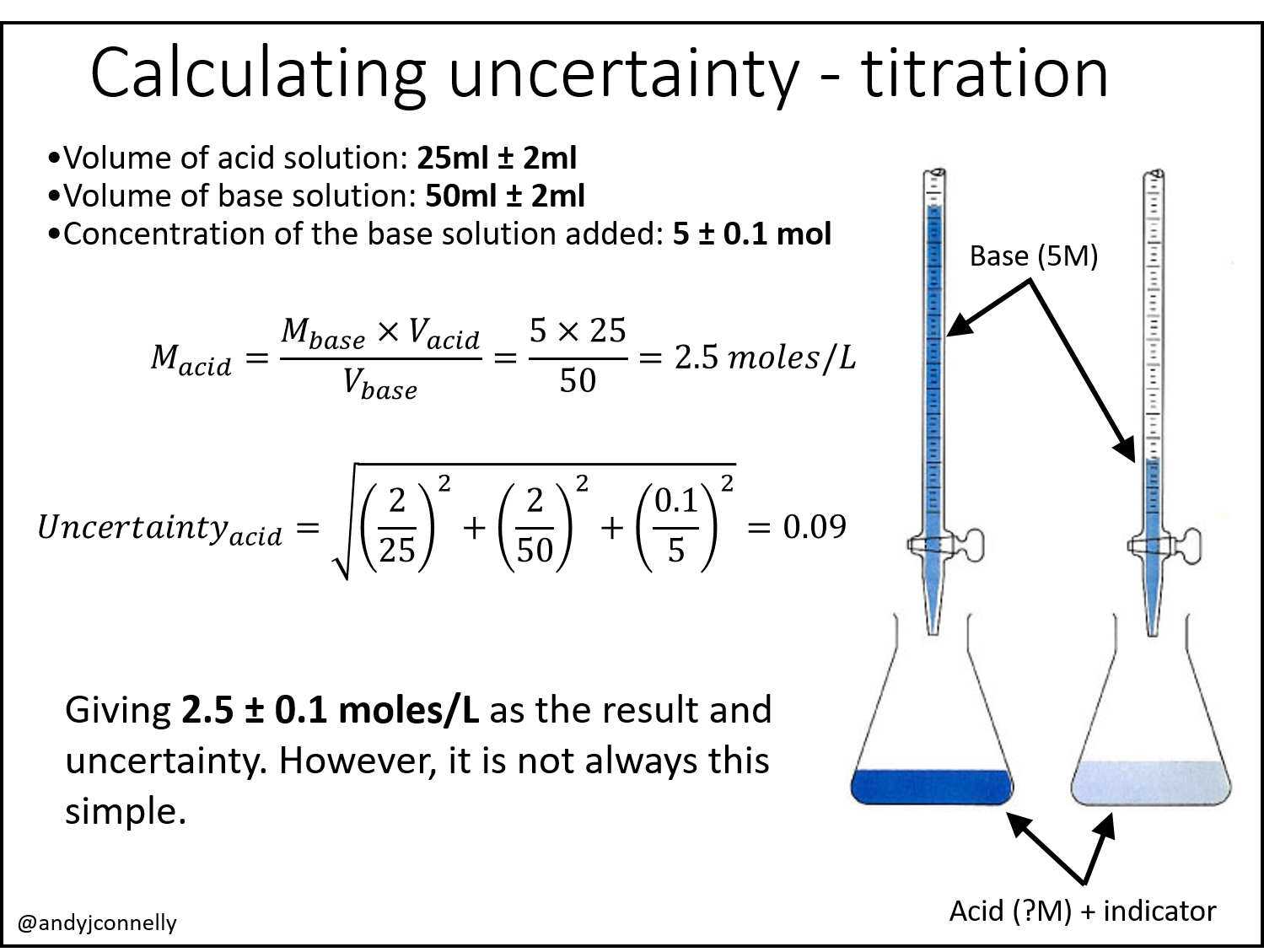
The reality of these types of calculations is that to take into account every aspect of the experiment that contributes error becomes rapidly impossible. Figure 2 shows an example of how seemingly simple experiments have a huge number of potential errors that need to be considered. Even the simple uncertainty calculation above for the acid-base titration becomes complicated given a full assessment of the potential errors.

This complicated process means that for most research purposes repeated measurements are an easier and quicker way of assessing the true uncertainty of a set of measurements.

Figure 2: Sources of uncertainties in an acid-base titration. Taken from EURACHEM/CITAC Guide, Quantifying Uncertainty in Analytical Measurement, Second Edition, QUAM:2000.1

Standard deviation

Using repeated measurements one of the first ways we learn to calculate uncertainty is through the standard deviation. This is a measure of spread of the data and has the same units as the quantity being measured.

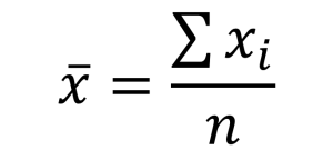
Equation for mean (where n=number of data points and xi is an individual data point)

Equatrion for mean (where n=number of data points and xi is an individual data point)

Equations for standard deviation. s=sample standard deviation and σ=population standard deviation.

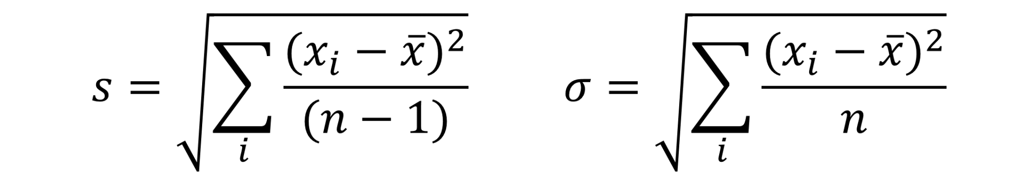
Unfortunately, standard deviation is of fairly limited use as the range of values being measured has a large impact on this value (see Table 1). Relative standard deviation can be used to partially solve this problem (see below). However, the most robust measure of uncertainty, for research, is usually the confidence interval.

Table 1: Different methods of measuring uncertainty have advantages and disadvantages.

All of the ways of representing uncertainty used in Table 1 are acceptable so long as you are clear what method you have used. However, if you are going to use standard deviation as a measure of uncertainty you should record it as, for example: “0.25ml (s=0.13ml and n=4)” [1].

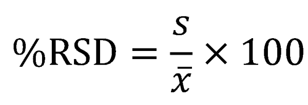
Relative Standard Deviation (RSD)

RSD (or %RSD) is widely used in analytical laboratories. It is a useful way of expressing uncertainty as it is easy to calculate and appears easy to interpret. People interpret percentages more easily than the standard deviation in units of, for example, mg/mL. Also, comparisons can be made across dissimilar results (particularly where the units of the measurements are different, for example ppm and absorbance). Less than 1% is usually considered very good for routine measurements which are more often in the 1-5% range.

%RSD does have disadvantages (see Table 1). The meaning of it is less intuitive than confidence intervals and the %RSD is not useful for data with a very small average. As the average gets smaller, the %RSD gets larger, approaching infinity as the average approaches zero, which is not a desirable result. Also, %RSD should only be used where zero for the measurement has real physical meaning such as length, weight, or area under the curve. Don’t use it where zero is arbitrary, such as pH.

If you are going to use %RSD then you should also report sample size, mean, and standard deviation.

Confidence intervals

For my mind, confidence intervals gives us the most robust idea of uncertainty. To quantify uncertainty in this way we need:

• Two or more measurements
• Sample mean
• Sample Standard Deviation
• t values table

Normal distribution

Confidence limits assume that your data take a Gaussian (normal) distribution as that shown in Figure 3. With only 5 or 6 data points you will not see this distribution but we have to assumed that if you repeated these measurements enough times this distribution would appear.

Be warned! Not all data fit this kind of distribution. If your data do not fit a Gaussian curve then none of the maths from this point will work! There are tests you can apply to your data to check it follows the normal distribution.

Figure 3: Data forming a Gaussian (normal) distribution.

Figure 4 shows the how the mean and population standard deviation are defined on these curves. These are defined:

• Mean: Mean (average) of a large set of data, units same as individual measurement.
• Population Standard Deviation: Measure of spread of a large set of data, Units same as individual measurement.

As can be seen in Figure 4 one standard deviation from the mean includes 68% of the data, two standard deviations from the mean includes 95% and three 99.7%.

Figure 4: Graphs showing the different proportions of the curves taken up by the population standard deviation and multiples of the population standard deviation.

• Confidence Interval: A range of values about a sample mean which is believed to contain the population mean with a stated probability, such as 95% or 99%. Gives robust uncertainty measurement. It is a measure of how confident you are that the result is within a specified range. This can be calculated using the normal distribution (see below) or the t-distribution (see next section) where you have only a handful of measurements.

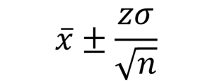
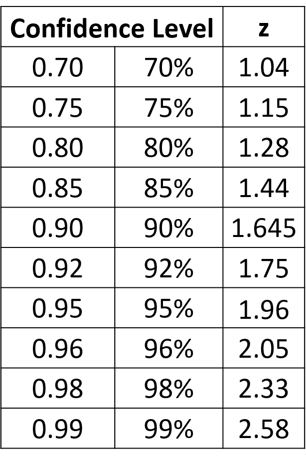
Below are the equations you can use if you are using the normal distribution for your uncertainty calculations (here z can be equal to values shown in Table 2). This is how we would make this calculation in an ideal world where you have lots and lots of data. See the next section for a more ‘real world’ approach.

Confidence intervals (normal distribution)

Confidence intervals (normal distribution) for a limited data set.

Table 2: Table of z-values for Confidence Intervals

So, for a 95% confidence interval if we repeated an experiment 100 times and checked to make sure there were no gross errors, 95 of the repeats would be expected to have results within the range of the confidence interval. Another way to say this is:

• the volume is 10ml±(1.96×1.5ml)=10ml±2.9ml at a confidence level of 95% (where n=5)

Or that:

• the 95% confidence limits for the volume are 10ml±2.9ml (n=5).
• The 95% confidence interval is 7.1 – 12.9ml (n=5)
• If I repeated this measurement 100 times 95 of the results would be in the range 7.1 – 12.9ml (n=5).

Student t-distribution

In real-world measurements we often do not have enough data points to form a normal distribution. We have to make an extra calculation, a calculation of the confidence intervals using a student t-distribution the Mean and the Sample Standard Deviation. This is normally taken to be the case with fewer than 20-30 measurements.

Figure 5: Exaggerated representations of the z and t distributions

These equations use the idea of Degrees of Freedom (DoF). In general, DoF is the number of terms in a sum minus the number of constraints on the terms of the sum. In this simple case the DoF is n, where n is the number of measurements you have made. When the mean of the measurements is defined then DoF becomes (n-1).

Using the equation in Figure 6 we can calculate the 95% confidence interval. This gives the range of values with a 95% confidence level. Table 8 shows the t values for different degrees of freedom required this calculation. For example (where n=5 and standard deviation=0.0311 litres)

Table 3: Values for student t that can be used to calculate confidence intervals. Values taken from uregina.ca/~gingrich/tt.pdf

Figure 6: Confidence interval calculation

• the 95% confidence interval for the volume is 9.97 – 10.05 L (n=5)
• The 95% confidence limits are 10.01 ± 0.04 L (n=5)
• with confidence level 95%, the true mean lies within the confidence interval

In the method section you could write:

• “The reported uncertainty is based on a t-distribution corresponding to a coverage probability of 95%.”

Summary

Reporting the uncertainty of your data is vital. Without this a reader has no idea as to the validity of your data. A difference of 3ppm between two measurements is meaningless if the uncertainty of the measurement is 10ppm. It is often a daunting prospect to repeat measurements but if you are clever with your experimental design it can be achieved with minimal extra effort. you don’t need to repeat every sample 6 times just key, representative samples.

References and further reading

[1] Data Analysis for Chemistry, Hibbert & Gooding, 2006.

• Statistics and Chemometrics for Analytical Chemistry, Miller & Miller, 5th ed. Pearson (2005)
• Statistics: A guide to the use of statistical methods in the physical sciences. Roger Barlow, John Wiley & Sons, 1989.